Deep Learning
Table of Contents
1 Introduction
Notes on my studies on Deep Learning techniques
2 Classes of Artificial Neural Networks
2.1 Recurrent Neural Networks - RNNs
A recurrent neural network (RNN) is a class of artificial neural networks where connections between nodes form a directed graph along a temporal sequence. source: Wikipedia
2.2 Convolutional Neural Networks - CNN
In deep learning, a convolutional neural network (CNN, or ConvNet) is a class of deep neural networks, most commonly applied to analyzing visual imagery. source: Wikipedia
2.3 Generative Adversarial Neural Networks - GANs
A generative adversarial network (GAN) is a class of machine learning frameworks designed by Ian Goodfellow and his colleagues in 2014.[1] Two neural networks contest with each other in a game (in the form of a zero-sum game, where one agent's gain is another agent's loss). source: Wikipedia
3 Basic concepts
3.1 Binary classification
- Use either 0 (cat) or 1 (non cat)
Given \((x, y) \:\vert\: x \in \mathbb{R}^{n_{x}}\), with m train examples: \(\{(x^{(1)}, y^{(1)}), (x^{(2)}, y^{(2)}),...(x^{(m)}, y^{(m)})\}\)
3.2 Logistic regression
3.2.1 Model
Given \(x\), want \(\hat{y} = P(y=1 \vert x), x \in \mathbb{R}^{n_{x}}\)
parameters: \(w \in x \mathbb{R}^{n_{x}}, b \in \mathbb{R}\)
output: \(\hat{y} = \sigma(w^{T}x + b)\), where \(\sigma(z) = \frac{1}{1 + e^{-z}}\)
In some implementation it is add \(x_{0} =1\), therefore \(x \in \mathbb{R}^{n_{x}+1}\) and:
3.2.2 Gradient Descent
output: \(\hat{y} = \sigma(w^{T}x + b)\), where \(\sigma(z) = \frac{1}{1 + e^{-z}}\)
Given \({(x^{(1)}, y^{(1)}), (x^{(2)}, y^{(2)})}\), want \(\hat{y}^{(i)} \approx y^{(i)}\)
Loss (error) funcion:
- Quadratic error (not used)
\begin{equation} \mathcal{L}(\hat{y}, y) = \frac{1}{2}(\hat{y} - y)^2 \end{equation} - Loss function
\begin{equation} \mathcal{L}(\hat{y}, y) = -(y\log{\hat{y}} + (1 - y)\log(1 - \hat{y})) \end{equation} - Cost function definition
\begin{equation} \begin{split} \mathbf{J}(w, b) & = \frac{1}{m}\sum_{i=1}^{m}\mathcal{L}(\hat{y}^{(i)},y^{(i)})\\ & =-\frac{1}{m}\sum_{i=1}^{m}\Big[y^{(i)}\log{\hat{y}^{(i)}} + (1 - y^{(i)})\log(1-\hat{y}^{(i)})\Big] \end{split} \end{equation} - Objective
Find w, b that minimizes \(\mathbf{J}(w, b)\)
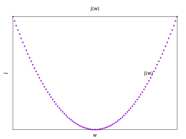
- Learning